Research CyberinfrastructureDivision of Information Technology · UW–Madison
Notebook 2 Cluster
Part 1: Continue with the Document
data-science
R
linguistics
pottery
aikido
brug
personal
productivity
coding
Quarto
reproducible research
research workflow
command line
Rscript
CHTC
portable code
data subsetting
toolero
A practical guide to starting a research coding project with a structure that can grow from local exploration to reproducible analysis, containerized execution, and high-throughput computing. Part 0 of the “From the Notebook to the Cluster” series.
Author
Affiliation
Erwin Lares
Research Cyberinfrastructure (RCI), Division of Information Technology, UW-Madison
Published
July 1, 2026
Modified
July 17, 2026
1 The long game
In Part 0, we gave the project a home. We created a project structure that was not only useful for local work, but also prepared for the later steps in this series: writing a reproducible analysis document, deriving a runnable script, containerizing the software environment, and eventually submitting the work to CHTC.
That order matters.
A project that starts with a stable structure is easier to reason about. Raw data has a predictable location. Results have a predictable destination. Future job inputs have a place to go. The analysis is no longer just a script somewhere on a laptop. It belongs to a project.
In Part 1, we create the document that will carry the analysis.
The point of this post is not simply that Quarto is a good reporting tool, although it is. The larger point is that a Quarto document can become the source of truth for an analysis. Prose, code, outputs, and decisions live together. From that document, we can derive the standalone .R script that later stages of the workflow will need.
That distinction is important for the long game:
.qmd document  -> human-readable source of truth
.R script      -> machine-executable derived artifact
The .qmd is where we explain the analysis. The .R file is what we will eventually run outside the document, containerize, and hand to a scheduler.
If those two files are maintained separately by hand, they can drift apart. If the .R file is derived from the .qmd, the relationship is clearer: edit the document, render the document, regenerate the script.
That is the role of toolero::create_qmd() in this workflow.
2 Where this post sits in the sequence
This series follows a deliberate path:
Part 0  create the project home     -> toolero::init_project()
Part 1  create the document/code    -> toolero::create_qmd()
Part 2  containerize the project    -> containr
Part 3  submit the first job        -> submitr single-job workflow
Part 4  submit many jobs            -> toolero::write_by_group() + submitr
Each step prepares for the next one.
In Part 0, we used toolero::init_project() to create a project called palmer-penguins-analysis. We also made one project-specific choice: because we know this analysis will eventually be split into job-sized inputs, we created data/jobs/ from the beginning.
At the start of this post, assume the project has this shape:
That path will appear throughout the post. The name is intentionally specific. A file called data.csv is convenient in the moment, but it becomes vague quickly. A file called palmer-penguins.csv tells us what the input is before we open it.
3 Why start with the document?
Most research projects start as a script. That is understandable. A script is direct. It lets you load the data, try an idea, make a plot, and keep moving.
The difficulty appears later.
A script can tell you what the code did, but it often does not tell you why the analysis was written that way. It may not record which decisions were exploratory and which became part of the final workflow. It may not explain why a particular input path, model, filter, or figure exists. When the project needs to be shared, reviewed, revisited, or moved to another machine, that missing context becomes expensive.
A Quarto document helps because it keeps the reasoning close to the code. The explanation, the executable code, and the outputs live in one place. The analysis is no longer a script plus a separate set of notes plus a folder of copied figures. It is a document that can be read, rendered, and inspected.
There is also a practical benefit that is easy to underestimate: consolidation. A common research workflow spreads the work across several tools: code in an editor, tables and charts in a spreadsheet, narrative in a document editor, and a manual copy-paste step connecting them all. Every time the data changes, the cycle repeats.
Quarto collapses much of that work into a single source. Tables and visualizations are generated directly from the code and appear in the document automatically. When the data changes, a render updates the outputs. There is no figure to re-export by hand and no table to manually reconcile.
This does not mean that every project should remain a single document forever. That would be too strong a claim. As a project grows, reusable functions may belong in R/, helper scripts may belong in scripts/, and long-running computation may need to move elsewhere. But as a starting point, the Quarto document gives the project a narrative spine.
The goal is not purity. The goal is to keep the analysis understandable, reproducible, and easy to move.
4 Create the document with toolero
The toolero package includes create_qmd(), a function that scaffolds a Quarto analysis document with reproducible project conventions in mind.
First, load toolero:
library(toolero)
From inside the project root, create the analysis document:
This does more than create an empty .qmd file. It gives us a starting document and, by default, sets up the mechanism that helps prevent code drift: a post-render purl() workflow that extracts the R code from the document into a companion .R script.
The important relationship is one-way:
edit the .qmd -> render the document -> derive the .R script
The .qmd is the file we maintain. The .R script is derived from it.
That is the design choice that matters. If we later run the script from the command line, inside a container, or as part of a CHTC job, we want confidence that the script reflects the current document. We do not want two parallel versions of the analysis that have to be kept in sync by memory.
5 Use YAML to make repeated setup less repetitive
A Quarto document begins with YAML metadata. At its simplest, YAML records the title, format, and other rendering options for the document. In practice, it often becomes a place where repeated setup accumulates: author name, affiliation, table of contents settings, theme, CSS, project-specific parameters, and other conventions.
This is one of the reasons create_qmd() is useful. If you regularly create documents with the same author information, institutional metadata, preferred options, or parameters, you should not have to rebuild those fields by hand every time.
create_qmd() can use a YAML configuration file to pre-populate the document header:
For this post, the key parameter is the input data file:
params:data_file:"data-raw/palmer-penguins.csv"
That parameter gives the document a default input when it is rendered with Quarto. Later, when the same code is run with Rscript, the input can be supplied as a command-line argument instead.
This is the beginning of portability. The same analysis can be run in more than one context without editing the code each time.
6 Before we write the analysis
Before writing analysis code, it is worth naming the constraints we want the document to satisfy.
The document should:
read the original dataset from data-raw/palmer-penguins.csv;
write tabular outputs to results/;
write visual outputs to plots/;
behave correctly when rendered as a Quarto document;
behave correctly when run as a standalone .R script;
make the later transition to containerized and scheduled execution easier.
Those are not advanced requirements. They are the normal requirements of a project that may eventually leave your laptop.
The safest time to account for them is now.
7 A minimal analysis thread
The analysis in this post is intentionally small. We will use the Palmer Penguins dataset to calculate summary statistics for flipper length and visualize the distribution of flipper length by species.
The analysis itself is not the point. The pattern is the point.
A small analysis lets us focus on the structure:
flowchart LR
  A[Load libraries<br>and data] --> B[Prepare data]
  B --> C[Calculate summaries]
  C --> D[Render table]
  C --> E[Render plot]
  D --> F[Save outputs]
  E --> F
flowchart LR
  A[Load libraries<br>and data] --> B[Prepare data]
  B --> C[Calculate summaries]
  C --> D[Render table]
  C --> E[Render plot]
  D --> F[Save outputs]
  E --> F
Figure 1: Analysis workflow
Figure 1 gives the bird’s-eye view. We load the data, compute summaries, render outputs, and save the deliverables in predictable locations.
That final step matters. A result printed to the screen may be useful during exploration, but a reproducible workflow needs files that can be inspected, shared, archived, or retrieved after a job runs somewhere else.
8 Resolve inputs across execution contexts
One of the subtle challenges in this workflow is avoiding code drift across execution contexts.
It is very easy to begin with one version of the logic for interactive work in RStudio, introduce a slightly different version for quarto render, and eventually add another version for Rscript when the analysis needs to run headlessly. Over time, those entry points can drift apart. A path gets updated in one place but not another. A parameter is handled differently. Behavior that worked locally no longer matches the rendered or scheduled version.
The result is duplicated logic and a project that becomes harder to trust.
The code below keeps the input resolution in one place. In an interactive session, the data path is convenient for local development. In a Quarto render, the path comes from the YAML params block. In an Rscript call, the path comes from the command-line argument, which is the pattern a job scheduler can use later.
library(tidyverse)
── Attaching core tidyverse packages ──────────────────────── tidyverse 2.0.0 ──
✔ dplyr     1.2.1     ✔ readr     2.2.0
✔ forcats   1.0.1     ✔ stringr   1.6.0
✔ ggplot2   4.0.3     ✔ tibble    3.3.1
✔ lubridate 1.9.5     ✔ tidyr     1.3.2
✔ purrr     1.2.2
── Conflicts ────────────────────────────────────────── tidyverse_conflicts() ──
✖ dplyr::filter() masks stats::filter()
✖ dplyr::lag()    masks stats::lag()
ℹ Use the conflicted package (<http://conflicted.r-lib.org/>) to force all conflicts to become errors
Rows: 344 Columns: 8
── Column specification ────────────────────────────────────────────────────────
Delimiter: ","
chr (3): species, island, sex
dbl (5): bill_length_mm, bill_depth_mm, flipper_length_mm, body_mass_g, year

ℹ Use `spec()` to retrieve the full column specification for this data.
ℹ Specify the column types or set `show_col_types = FALSE` to quiet this message.
The important thing is that data_file is resolved once. The rest of the analysis does not need to know whether the code was run interactively, rendered as a document, or called from the command line.
That is a small design decision, but it has a long reach. It is one of the things that makes the .qmd and the derived .R script portable.
9 Tabular results
We can now calculate a small set of summary statistics for flipper length across the three penguin species.
The code below groups the data by species and computes the minimum, maximum, mean, and standard deviation of flipper_length_mm. The resulting data frame is then formatted as a table with gt when the document is rendered or run interactively.
Table 1: Summary statistics for flipper length by species
Flipper Length by Species
Summary statistics in millimeters
species
min_flipper_length
max_flipper_length
mean_flipper_length
sd_flipper_length
Adelie
172
210
190
7
Chinstrap
178
212
196
7
Gentoo
203
231
217
6
Table 1 shows a familiar pattern in the Palmer Penguins data: Gentoo penguins have longer flippers than Adelie and Chinstrap penguins. The table is useful because it makes the numerical pattern explicit.
For the long game, there is another point worth noticing. The object flipper_stats is not only something we can print in the document. It is also something we can save as a file.
That distinction matters when the analysis runs outside the document.
10 Visualizing distributions
A table summarizes the pattern, but a plot makes the distribution easier to inspect.
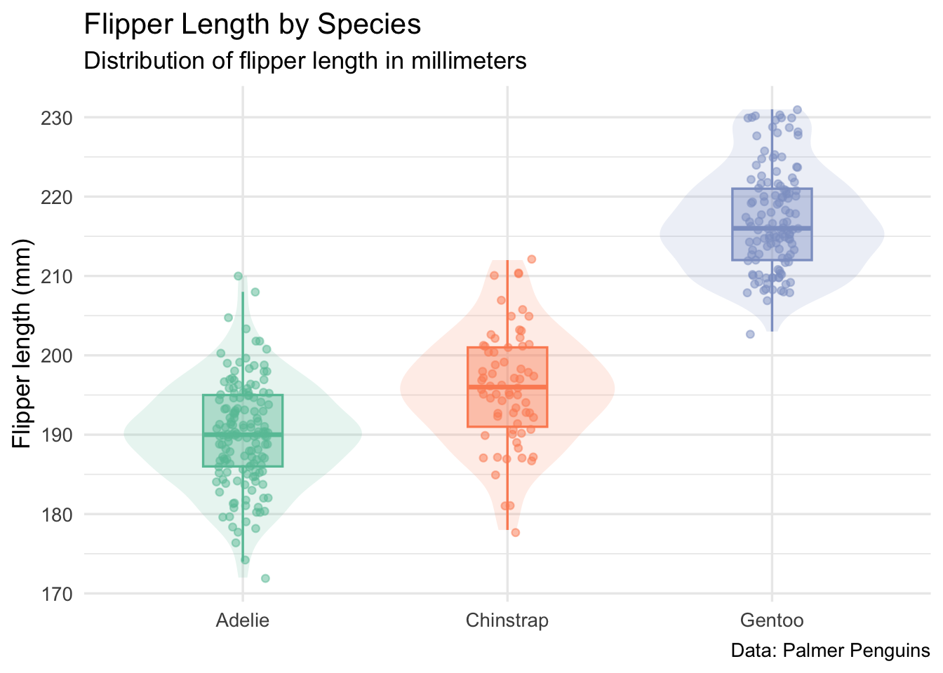
The code below visualizes flipper length across species using three complementary layers: a violin plot for the distribution, a boxplot for the summary, and jittered points for the individual observations.
p <- data |>ggplot(aes(x = species,y = flipper_length_mm,color = species,fill = species )) +geom_violin(alpha =0.15, linewidth =0) +geom_boxplot(alpha =0.4, width =0.3, outlier.shape =NA) +geom_jitter(width =0.1, alpha =0.5, size =1.5) +scale_color_brewer(palette ="Set2") +scale_fill_brewer(palette ="Set2") +labs(title ="Flipper Length by Species",subtitle ="Distribution of flipper length in millimeters",x =NULL,y ="Flipper length (mm)",caption ="Data: Palmer Penguins" ) +theme_minimal(base_size =13) +theme(legend.position ="none")if (should_render_outputs) p
Warning: Removed 2 rows containing non-finite outside the scale range
(`stat_ydensity()`).
Warning: Removed 2 rows containing non-finite outside the scale range
(`stat_boxplot()`).
Warning: Removed 2 rows containing missing values or values outside the scale range
(`geom_point()`).
Figure 2: Distribution of flipper length by species
Figure 2 shows the same general result as the table, but with more texture. Adelie and Chinstrap penguins overlap more strongly, while Gentoo penguins are visibly larger by this measure. The point is not that this is a complicated analysis. The point is that the document lets us keep the explanation, code, table, and plot together.
11 Save analysis outputs
In many analyses, the deliverables are not only objects printed to the screen. They are files saved for later use: summary tables, plots, model objects, logs, or other artifacts that a collaborator, manuscript, or later workflow will need.
For this project, the folder conventions were established in Part 0:
results/   # tabular or non-visual outputs
plots/     # visual outputs
The code below saves the summary statistics to results/ and the plot to plots/.
This is a modest step, but it is a useful habit. The script does not assume that a person will manually create output folders before running it. It checks for the directories it needs and writes deliverables to predictable locations.
That matters later, when the same code runs without anyone watching it.
12 Derive the runnable R script
When the analysis needs to run at scale, the document-rendering overhead may be unnecessary. At that point, we want the code, not the narrative.
This is where create_qmd() does more than create a blank Quarto document.
By default, create_qmd() can set up the project so that rendering the .qmd also derives a standalone .R script from the document. That behavior is controlled by the use_purl argument.
With use_purl = TRUE, toolero creates the pieces needed for an automatic post-render workflow. The project gets a _quarto.yml file that registers a post-render hook, and that hook runs a purl.R script after the document renders.
Conceptually, the workflow looks like this:
render the .qmd
  -> Quarto reads _quarto.yml
      -> post-render runs purl.R
          -> purl.R derives the companion .R script
The result is the same relationship we want for the long game:
You maintain the .qmd. The .R script is regenerated from it.
Under the hood, the post-render script relies on knitr::purl(), which extracts R code chunks from a literate document and writes them to a standalone script. The source template for that helper script lives in the toolero package at inst/templates/purl.R. When create_qmd(use_purl = TRUE) is called, toolero copies or writes the needed post-render helper into the project so the project can regenerate its own .R script when rendered.
The exact implementation detail is less important than the direction of authority:
.qmd is maintained by the researcher
.R is derived by the project machinery
That direction is what prevents code drift. If the document and the script are both edited by hand, they can become two similar but different analyses. If the script is derived from the document, the relationship is clearer: edit the document, render the document, regenerate the script.
The .qmd is the source of truth. The .R file is the derived artifact.
13 Prepare for job-sized inputs
At this point, we have a document that can render an analysis and save outputs. That is enough for a local workflow. It is not yet enough for a high-throughput workflow.
HTC becomes useful when a larger task can be split into many independent pieces. For this toy example, splitting by penguin species is not computationally necessary. It is useful because it illustrates the pattern we will need later: one input file per job.
In Part 0, we created data/jobs/ for this future purpose. Now we can use it.
toolero::write_by_group() splits a data frame by a grouping column, writes one CSV file per group, and optionally writes a manifest that records the files created.
✔ Written "Adelie" (152 rows) to 'data/jobs/adelie.csv'
✔ Written "Chinstrap" (68 rows) to 'data/jobs/chinstrap.csv'
✔ Written "Gentoo" (124 rows) to 'data/jobs/gentoo.csv'
✔ Manifest written to 'data/jobs/manifest.csv'
This gives the future submission workflow a set of job-sized inputs. Conceptually, the structure is now:
data-raw/palmer-penguins.csv   # original input data
data/jobs/                     # split inputs for later jobs
The raw data remains untouched. The job inputs are derived from it.
That distinction is worth preserving.
14 Run the derived script from the command line
Once the .R script has been generated and the data has been split into subsets, each subset can be processed independently by passing it as a command-line argument.
This is the same kind of call that a job scheduler can use later. At small scale, you run one command manually. At larger scale, a submit file runs the same script many times, each time with a different input file.
The fact that the same script can run in both situations is the point. The portability was built in earlier, when we resolved the input file based on the execution context.
When the time comes to scale, the transition should be a change in infrastructure, not a rewrite of the analysis.
15 What we have after Part 1
At the end of Part 1, the project has moved from a structured home to a structured analysis.
We now have:
a Quarto document that explains the analysis;
a derived .R script that can run outside the document;
an input path that works across interactive, Quarto, and Rscript contexts;
a summary table saved under results/;
a plot saved under plots/;
job-sized input files saved under data/jobs/;
a pattern that can be containerized and eventually submitted to CHTC.
The important thing is not that the Palmer Penguins analysis is complex. It is not. The important thing is that the project now has a shape that can move.
16 What comes next
In Part 2, we will turn to the software environment.
Running a script outside the document is one step. Running it somewhere other than your laptop is another. For that, the project needs a portable software environment: the right R version, the right package versions, and the system libraries those packages require.
That is the role of containr.
The project already has the pieces that make containerization easier: a stable project structure, a clear input path, a derived script, saved outputs, and an renv.lock file. In the next part, we will use those pieces to build a container image.
For now, the document is doing what we need it to do.
It explains the analysis for humans and produces a script that machines can run.